Advanced XLOOKUP Tricks: Searching Multiple Criteria Like a Pro

The Problem: Beyond the Simple Lookup

Imagine you have a sales table. You want to find the "Commission" for a specific "Sales Rep" but only for a specific "Region."

A standard XLOOKUP only looks for one value. To find both, most people create "Helper Columns" (merging Rep + Region), but that’s messy and inefficient. In the Smart Sheet Lab, we prefer a cleaner, more elegant formula.

The "Boolean Logic" Solution

To search with multiple criteria, we use the power of 1 and 0 (True and False). Instead of searching for a text string, we tell Excel to look for the number 1 within a set of conditions.

The Formula Anatomy:

=XLOOKUP(1, (Criteria_Range1=Criteria1) * (Criteria_Range2=Criteria2)* (...), Return_Range)

Step-by-Step Breakdown

1. Setting the Target

We set the lookup_value to 1. Why? Because when we multiply conditions in Excel, "True" equals 1 and "False" equals 0. We want to find the row where all conditions are True.

2. Defining the Criteria Arrays

Let’s say:

• Condition 1: A2:A10 = "John" (Returns an array like {True, False, True...})

• Condition 2: B2:B10 = "Male" (Returns an array like {True, True, False...})

3. The Multiplication Magic

When you multiply these two arrays (Range1=Criteria1) * (Range2=Criteria2)* (Range3=Criteria3), Excel performs the math:

• True * True = 1 (A Match!)

• True * False = 0

• False * False = 0

Excel now looks through that resulting array of 1 and 0, finds the 1, and returns the corresponding value from your return_range.

A Real-World Lab Example

You have a sale list:

• Column A: Date

• Column B: Salesperson

• Column C: Item

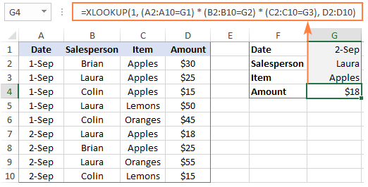
You want to find the mount of a "Apple" that is sold by "Laura" on "2-Sep".

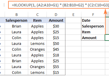
The Smart Formula:

=XLOOKUP(1, (A2:A10=G1) * (B2:B10=G2) * (C2:C10=G3), D2:D10)

Why This Method is "Lab-Grade" Superior

1. No Helper Columns: Keeps your data structure clean and professional.

2. Infinite Criteria: You aren't limited to two. You can add a third, fourth, or fifth condition just by adding another * (Range=Criteria) block.

3. Dynamic: It works perfectly with Table References (e.g., Table1[Product]), making your spreadsheets future-proof.

Pro Tip: Handling "Not Found"

One of the best features of XLOOKUP is the built-in error handling. Don't let your dashboard break with an #N/A. Always add the "if not found" argument:

=XLOOKUP(1, (A2:A10=G1) * (B2:B10=G2) * (C2:C10=G3), D2:D10, "No Match Found")

Final Lab Report

Mastering multiple-criteria XLOOKUP is a rite of passage for any Excel expert. It moves you away from "basic spreadsheets" into "data engineering." Practice this logic, and you’ll find yourself building tools that others thought were impossible in Excel.